Google ASL Fingerspell Kaggle Challenge
designing, training, and deploying a seq2seq model that estimates sign language from pose estimates
This was my submission to Google's ASL Fingerspell Challenge. It's not much and I still clearly have a long way to go before I can call myself an expert at this stuff. That said, I am proud of my work here and I don't think there have been many other times where I have learned this much in such a small amount of time. Because it is my first real deep learning project, this summary will be more in-depth than just a showcase. I try to recount all of my main challenges and learnings that came out of the engineering/research process. I also shouldn't go any further without thanking the couple of folks who provided their experienced advice when I needed their guidance. Know that your advice went a long way, helping me push through some of the moments of doubt and uncertainty in this.
The code for the project can be found here
Without further ado, the writeup has the following structure
- Primary tasks
- Processing and loading a ~200G tabular dataset efficiently
- Setting up cloud training and file storage infrastructure
- Designing and training a seq2seq model that converts vector time-series data into text
- Guiding engineering principles
- How to scale up
- Model iteration
- Further research
- Transfer learning with character-level language models
Primary tasks
Dataset preprocessing and loading
You can get a more formal of this competition description by reading the Kaggle competition page, but here I will give a condensed version of the task here. You are given a set of 3d landmarks generated by Google's MediaPipe library against a set of subjects performing ASL fingerspell motions. These data are represented in a 2-dimensional table of column-labeled time series. Associated with each sequence is the correct text label in latin alphanumeric text (59 character classes) which have no alignment with the sequence time frames. The task is do design a model that can predict these character text labels. The evaluation metric of the model is the normalized Levenshtein edit distance.
The first thing that struck me in this challenge is how hard it is to work with tabular data. Intuition would lead you to believe the opposite; working with standard format data like audio or image files has significantly more library overhead. I mean just try looking up how to parse a jpeg using the standard libjpeg methods. No, thank you! While that may be true, there are usually only one or a couple different formats that are used to store these types of data due to their uniformity. There are therefore many nice frameworks like torchaudio, tensorflow vision and so forth have been built to abstract almost all of that format wrangling away. In the end, you have to do almost no work between pointing an image loading call at a file name and having a torch tensor ready to go in just milliseconds.
Tabular data has a different story because it is such a flexible format. There are many ways in which it can be stored natively: CSVs, parquets, binary records with another layer of encoding, excel spreadsheets (if that finance bro friend of yours has asked you to do some of that "coding stuff"), etc. You can probably name at least a few more popular ones. At the end of the day, there's a reason why data engineers exist and that is to perform this task that no library can do comprehensively.
We are dealing with vector time series data in this task, which were all generated by a pose estimation model that has something like 543 landmarks that it estimates on a subjects' body. One can visualize this in an excerpt of the left hand in one training example:
There is a sort of relational schema to this competitions training data. You have a manifest file and a set of parquet files. The manifest contains a list of all the training examples, their labels and some metadata pointing to their location in the parquet files. Each parquet contains some number of vector time series indexed by the sequence id given in the manifest. Have a look:
Train.csv
<div style="overflow-x:auto">
| path | file_id | sequence_id | participant_id | phrase |
|---|---|---|---|---|
| ./5414471.parquet | 5414471 | 1816796431 | 217 | 3 creekhouse |
| ./5414471.parquet | 5414471 | 1816825349 | 107 | scales/kuhayla |
</div>
5414471.parquet
<div style="overflow-x:auto">
| sequence_id | frame | x_face_0 | x_face_1 | ... |
|---|---|---|---|---|
| 1816796431 | 0 | 0.710543 | 0.699916 | ... |
| ... | ... | ... | ... | ... |
| 1816825349 | 0 | 0.325671 | 0.841324 | ... |
</div>
There are a couple of issues with using this storage format directly with your training pipeline. Size is one. The parquet files, although they are a binary format, are chunked into files that are very large, take a long time to load and leave a large memory footprint during training. Furthermore, the number of raw features, 1,629 is intuitively high for a model that is just translating fingerspell sequences. We may want to hold off on this intuition because feature pruning is usually something done during training iterations, but it is worth a thought at this point.
At the start of this project, to cram the maximum number of preprocessing steps I could think of into this stage: coordinate centering, standardization, dimensionality reduction... whatever seemed like I could use, it was probably in my first preprocessing pipeline. I have this bias towards reducing any computational overhead that I see, one of the pitfalls of many novice engineers, and my preprocessing pipeline was an obvious expression of this. Having completed this part of the project, I now know there is a general rule of thumb one can follow to avoid this tendency in the data pipeline. Data should be preprocessed and stored with as much decoupling from the pipeline as possible. If you anticipate wanting to use your full feature set in the training stage, then don't do any feature selection or dimensionality reduction. The extra three dollars you'll save in monthly S3 storage fees is just not worth it lol. Take it from me as I learned during this project.
Okay, enough talk. Let's get into the nitty-gritty of how to store this data in the filesystem. You want to choose a scheme that aligns closely with how you plan to load the data during training and validation. If you are using a k-folds validation scheme, you'll probably want to partition the actual files into folds so that samples can be accessed in an independent, shuffled manner within their fold. If you look at asl_data_preprocessing.ipynb, you'll see that the file names are prefixed with a fold{n}, which is how I accomplished this. We then choose a binary format for storing the files. If you are training your model in TensorFlow, I strongly recommend that you use the library's TFRecord framework. Most will underestimate the life-changing impacts of using an integrated binary data storage like this baby. But, if you are willing to take my words of wisdom as a complete newbie to deep learning, this is absolutely the case. When your dataset is stored as TFRecords, you can do parallel reads in your dataloader, you can point your file addresses to google storage objects (stay tuned for the cloud infrastructure section), you can shuffle your otherwise iterable dataset using a variable-length shuffle buffer. It's literally all done for you in the TF library. For this reason alone, I went against the advice of all my more experienced friends and tried rewriting this entire project for TensorFlow. Honestly, it was not a mistake.
You can see that in the following, these are the only utilities you need to get your dataset written in the preprocessing stage and loaded in the training stage. Very simple, no boilerplate.
def encode_example(sequence: np.ndarray, frame: np.ndarray):
    feature = dict()
    feature['sequence'] = tf.train.Feature(bytes_list=tf.train.BytesList(value=[sequence.tobytes()])),
    feature['frame'] = tf.train.Feature(bytes_list=tf.train.BytesList(value=[frame.tobytes()]))
    return tf.train.Example(features=tf.train.Features(feature=feature)).SerializeToString()

def decode_example(b):
    features = dict()
    features['frame'] = tf.io.FixedLenFeature([], dtype=tf.dtypes.string)

    features['sequence'] = tf.io.FixedLenFeature([], dtype=tf.dtypes.string)

    decoded = tf.io.parse_single_example(b, features)
    decoded['frame'] = tf.reshape(tf.io.decode_raw(decoded['frame'], tf.dtypes.float32), (-1, N_FEATURES, 3))
    decoded['sequence'] = tf.io.decode_raw(decoded['sequence'], tf.dtypes.int64)
    return decoded

  # to write a chunk of examples, we use a utility like the following
def write_chunk(data, write_dir, chunk_num):
    (frames, seqs), fold = data
    chunk_size = len(frames)
    filename = os.path.join(write_dir, f'fold{fold}-{chunk_num}-{chunk_size}.tfrecord')
    options = tf.io.TFRecordOptions(compression_type='GZIP')
    writer = tf.io.TFRecordWriter(filename, options=options)
        for frame, sequence in zip(frames, seqs):
            encoded_bytes = encode_example(sequence, frame)
            writer.write(encoded_bytes)
        writer.close()

  # then when we want to load a dataset, we just have to map our decode function to the dataset
ds = tf.data.TFRecordDataset(['fold0-0-256.tfrecord', 'fold0-1-256.tfrecord', ...], compression_type='GZIP')
ds = ds.map(decode_example)
The way to do something like chunked parallel loading datasets in PyTorch is a little bit more involved, but as is usual with the PyTorch/TensorFlow matchup, you trade off library conformity and a lot of pre-designed features for flexibility. Looking back on this project now, I do prefer the PyTorch method a little more because it encourages you to understand how your project is engineered as opposed to how to get TensorFlow to do what you want. The following is just a dataset of random normal floats and uniform integers that demonstrates how you can store associated features and labels with torch.save. Again, if you want to use worker processes to do the loading, you'll have to implement this yourself as PyTorch doesn't have any of those utilities
n_sequences = int(1e6)
max_seq_len = 384
min_seq_len = 50

max_label_len = 30
min_label_len = 10

n_features = 1630
n_tokens = 59

sequence_lengths = torch.randint(n_sequences, min_seq_len, max_seq_len)
label_lengths = torch.randint(n_sequences, max_label_len, min_label_len)

# sorry about the for loops, this formatter doesn't support list comprehension
data = dict()
for i in range(n_sequences):
    example = dict()
    example['sequence'] = torch.randn((sequence_lengths[i], n_features))
    example['label'] = torch.randint(label_lengths[i], 0, n_tokens)
    data[i] = example

chunk_size = 256
for chunk in n_sequences // chunk_size:
    chunk = dict()
    for i in range(chunk_size):
      chunk[i] = data[chunk*chunk_size + i]
    torch.save(chunk, f'chunk{chunk}.pt')
Cloud training and storage resources
I had some prior experience with provisioning cloud resources going into this project. The part of this project that arguably would have had the steepest learning curve---figuring out how the heck to get your AWS service accounts to authenticate on remote instances---was already sort of done for me.
😎
It was still valuable to spend my time on getting familiarized with the various AI training and deployment tools that the big cloud platforms these days have to offer. The obvious three demands that you have for your cloud platform are file storage for your training data, compute for training, and finally a container service for running deployments. In my familiarity with AWS, I was already acquainted with the S3, EC2, and ECR+ECS workflow. I tried sticking with what I knew about these platforms, avoiding having to use the extra bells and whistles of the SageMaker platform. It turns out that this is very hard for a one-off project where you have to setup all environments by yourself and provision the right EC2 instance hardware to match your training needs. After waiting for 5 days to get my provisional request approved for a g4dn.xlarge instance, my patience had reached its end. It was becoming evident that trying to walk this path would easily double the amount of work required by the project. I decided to either pivot to SageMaker or an entirely new cloud platform.
Everyone who knows anyone who codes has probably used Google Colab once or twice before. While there are some painful things about the platform, most notably its weird and unpredictable policy of hardware provisioning, I now realize that it is an insanely good free resource for most of these entry-level ML projects. They give you a 12-hour connection, albeit with spotty coverage, to a TPU V4 instance. For reference, SageMaker's cheapest tier at $0.74/hour runs on an EC2 ml.g4dn.xlarge instance, sporting a Nvidia T4 tensor core and 16 GiB memory which you can spec here. Maybe I'm penny-pinching to prefer not paying several dollars for each training run, but consider that you will be running your training notebook 20-100 times if you're as new to this as I am. Colab is also the platform on which the Kaggle notebooks run, which was an obvious vote in favor of Google's platform. That list made the decision for me and I didn't really have any doubts in other stages of the development process.
I mentioned before that TensorFlow's dataset objects support the gcloud storage protocol natively as file objects. This is awesome because you don't have to manage any of the file downloads in your own code. Cloud storage file access is also quite fast and was never a bottleneck during any of my training pipelines. I assume the fact that all of my resources were in Google Cloud helped with this.
Later down the line, I used Artifact Registry to upload the Docker images containing my trained models. This would have been significantly easier had there not been so much old documentation and writing that references the GCR platform which now no longer exists. With that all set in place, spinning the containers up in Cloud Run was a breeze.
This marks the end of the cloud tools section of the project. Most of the work here was bare-bones and I would not expect to be doing something this simple in an industry-level job. Perhaps for my next project where I do ML deployments, I will try something like building a pipeline for continuous training on new data or load-balancing on the containers deployments.
Model design
At this stage, you can take of your software and data engineering hat and put on your new generative AI hype PhD research transfer learning pants to try and build the next market-transforming neural network architecture. Well, to be a little more realistic, this stage is just about understanding the task and how it can relate to another problem that has been well-explored in research and industry. This should be a sufficient challenge alone.
It makes sense to understand the constraints of our model, considering a factor of increasing significance is model scaling---that is, many models have performance that scales with parameter counts. In this respect, we want to focus on a model that can perform optimally within these constraints. For this specific competition, the model must use less than 40Mb of storage in its disk representation. This gives us an upper bound of 40 million f32 parameters, which is intuitively high given the complexity of our application. For reference, AlexNet has 60 million parameters consisting of 5 convolution layers and 3 fully-connected. It was performant on recognition tasks for 256x256 images.
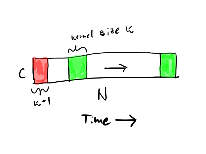
Considering our application, we want to perform a seq2seq task on vector time-series data where the input sizes are somewhere between 100 and 1000 time-steps of 100-200 dimension vectors. Many jump at the mention of seq2seq in language with the thought of an RNN or transformer architecture. However, consider a subtask where we are looking at frozen frames of a fingerspell sequence. Labeling a single character using a single time step or a window around a given time step should be possible. Moreover, it should be the fundamental subtask that we want our model to be good at performing. The lack of any long-term dependence in sequence steps means that the strengths of these two architectures are more or less irrelevant. The 1D CNN, on the other hand, makes a strong assumption about the correlation between near-time events which works to our advantage. This was also the primary architecture employed by many of the top-performing models in the ASL Kaggle Isolated Sign-Language Recognition competition.
I did some reading into how 1D CNNs are used for processing time-series and came across some articles about causal 1D CNNs, in which convolutions do not violate the principle of time-dependence. This may not seem important if the framerate of the sequences is very fast relative to the convolution kernel's length, but I did end up playing with the length parameter later in training to find that this feature did unlock a fair amount of performance. In implementation, causal 1D convolution requires padding of the input sequence with a block of zeros as long as the convolution kernel and then restricting the kernels's application to only valid portions of the input sequence (ie. no convolution over the edges). This is easy to visualize and in implementation, it is not that difficult either.
class CausalConv(tf.keras.layers.Layer):
    self.padding = tf.keras.Layers.ZeroPadding1D(padding=(kernel_size - 1, 0)
    self.conv = tf.keras.layers.DepthwiseConv1D(kernel_size, padding='valid')

def call(self, x):
    x = self.padding(x)
    x = self.conv(x)
    return x
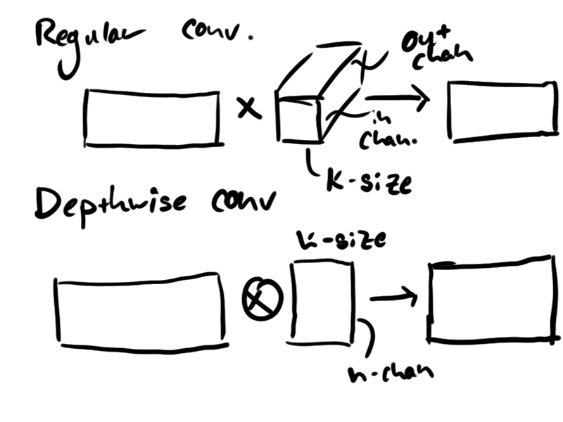
Once the first convolution has been applied to all channels, we encounter a lot of redundant crossing of channels if we continue to do full convolutions for all of the subsequent channel operations. This is the main principle behind depthwise convolution, which I think is a fairly standard operation in CV because both PyTorch and Keras have their own layers for the operation. I read the papers with code which had a great summary of how this has evolved in the field since fairly recently in 2016. In a 1D context, you can think of the depthwise convolution as a pointwise dot product between each channel in your input and a k-length vector in your kernel. We get to perform the operation without the extra output channel-length dimension in the convolution kernel, which is a significant reduction in the number of model parameters and the complexity of this operation.
Another mechanism that I came across which seems to result in small but global performance improvements is the channel-attention mechanism. Like an attention mechanism, the channel-attention mechanism learns to attend to various channels in the input based on features that it detects. Where in embedded word vectors, we do this between token embeddings, channel attention mechanisms detect features in their channels through pooling. The advantage of the efficient channel attention mechanism proposed by Wang, et al. in 2019 is that the attention is performed by a 1D convolution across the channel pooling. The assumption here is that attention features tend to occur in groups and that by convolving, you can encourage a spatial organization of these groups inside the attention mechanism. The operation that is performed looks a little like the following:
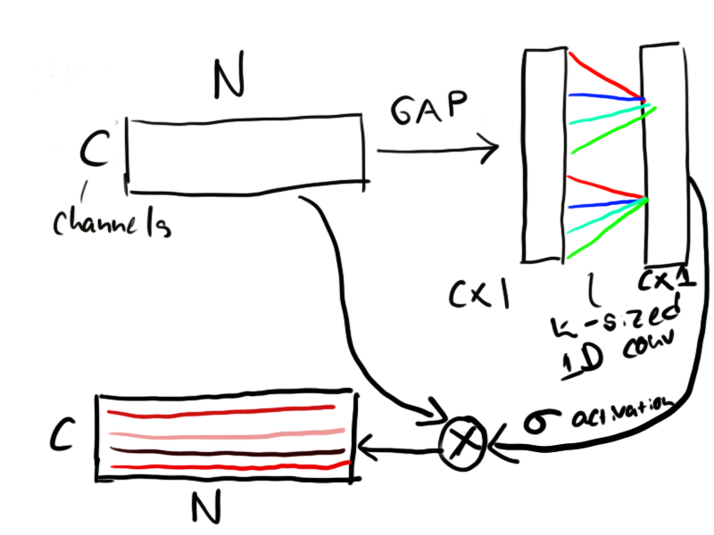
Implementing this as a neural net module is straight-forward: global average pooling is first performed along the last axis, we then have to reduce the empty axis before performing the convolution, we apply activation and finally, we perform the channel-wise multiplication with the input tensor:
class ChannelAttention(tf.keras.layers.Layer):
    '''An efficient channel attention mechanism as described in https://arxiv.org/abs/1910.03151'''
    def __init__(self, kernel_size=5, **kwargs):
        super().__init__(**kwargs)
        self.supports_masking = True
        self.gp = tf.keras.layers.GlobalAveragePooling1D()
        self.conv = tf.keras.layers.Conv1D(1, kernel_size=kernel_size, strides=1, padding='same', use_bias=False)

    def call(self, inputs, mask=None):
        nn = self.gp(inputs)
        nn = tf.expand_dims(nn, -1) # unsqueeze along last axis
        nn = self.conv(nn)
        nn = tf.squeeze(nn, -1)
        nn = tf.nn.sigmoid(nn)
        nn = nn[:,None,:]
        return inputs * nn
That about sums up the main mechanisms used in the repeated convolution blocks of this model. You can see the final implementation in the notebooks that are in the github repository linked at the top of the writeup.
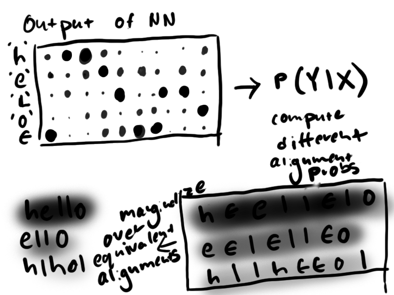
In sum, the NN computes a probability for each character at each time step of the input sequence. What would be nice is if the labeled data was aligned to the input sequences through time but it is not. All we have is a label of what these probabilities should predict if we collapse the time axis and take the changes in predicted token. This seems like a daunting task, but it is one that people have encountered for decades in optical character recognition and speech transcription tasks. They have developed a unique loss function that does just this called Connectionist Temporal Classification, or CTC. What CTC does is it computes the log probability of the loss Y given the NN output X probabilities log(P(Y | X)). It does this by marginalizing across all possible alignments of the input with the output using dynamic programming similar to the Viterbi algorithm for computing HMM probabilities. If you've never heard of this before, you are probably wondering how the algorithm handles repeated characters in text. Well, the loss algorithm expects that your network has also learned to predict an empty token ϵ in addition to the working tokens of the training set. Where the network predicts ϵ, the inference stage will just remove that token from the output. The following illustration shows at a high level how CTC loss is evaluated for P('hello' | X).
Note: there are serious problems that one can encounter with the numerical stability of CTC loss and long input sequences. I certainly had my fair share of trouble debugging convergence with this loss function. That topic deserves an article in itself, and I hope to put something out soon on that.
A note on masking
A final thing that one must consider when doing sequence alignment with text is how to handle variable-length inputs with batched training data. My intuition was just to pad the inputs to a max length and then I assumed that the neural network could learn the paddings to be sort of an end of sequence label. However, as the winner of the ASL isolated competition notes in their submission, this was something to avoid. This is just another labeling task that we are putting on our network and sure, maybe it can learn to label these pads correctly. However, if we can prevent the network from having to discern between these two types of data, we get much faster convergence as the gradients are no longer computed on these pad tokens.
Designing these modules thus required a bit of extra work to ensure that masking was supported, but this actually resulted in noticeable performance improvements across training runs. I eventually want to go back to measure just how significant those were and report them in this section of the article.
Guiding engineering principles
In this section, I go over some of the big-picture principles that I discovered in this project and ones that I think will guide my work on future machine learning projects. If you're tired of reading at this point, go outside and get some exercise or give your eyes a rest. The following points are rather strategic, maybe obvious stuff to most. But if you are interested, then please read ahead because I do see these as the most valuable takeaways for someone new to the game.
Project construction: how to scale up
When I first hear the word 'pipeline', I think the best way to build one is to follow the flow of data. This paradigm is strong in software engineering and it is mostly justified there because people work with very standard constructs like REST APIs, microservices and the like. Here, there is much less of a framework that each processing stage fits into, meaning there is a lot more decision-making that an engineer will have to make concerning the handoffs at each stage. Back to my initial approach, I worked in a linear, segmented fashion. I started out with the preprocessing, then got to the feature loading, I provisioned the cloud resources, etc. until I finished with the last stage and tried doing a training run. There is one large problem with this approach. How you design something in one stage affects the data that is ingested by all subsequent stages. This meas that if I make a major oversight in stage one, I may not realize that I have messed up until the final step when I think I am about to be all set and done. In an ML project where there are a lot more design decisions that affect the function of your pipeline, this is a concern.
A simple example of this was feature pruning. Feature pruning usually happens before the data is fed to the model and in that case, it was one of the first things I tried to engineer. When it came time to run training loops, I already had a frozen set of features sitting in cloud storage that needed to be reprocessed if I wanted to try training on a different feature set. I had not even considered the fact that I might want to try running a training iteration on the pose and face points in addition to the hand ones. This meant that significant work had to go into reimplementing that feature in every other stage of the pipeline (literally every other stage). The argument here is not that I should have engineered more things on the first iteration of this project. It is quite the opposite, actually. I should have instead focused on building an end-to-end system that satisfied the minimum constraints of the problem statement. Having this base system in place makes so many things easier because building the model incrementally is how one runs experiments. Nobody in their right mind can expect to select the right architecture or network sequence on the first iteration of their work.
Model iteration
That transitions into the discussion of how you improve performance through experimentation and consulting literature. If the last section was a slight difference between building ML models and more traditional software engineering, then this one is where the two disciplines truly depart from one another. It is likely the reason why I enjoy this type of work more, as well.
There will come a stage where the scaling in your project transitions from high-level, foundational questions like "how do I want to distribute my model training?" to much more direct and oftentimes mathematical questions about why your system behaves the way it does. The most effective way to start answering these questions is just to start iterating on potential solutions and improvements. Software engineering sometimes tells you that this is a bad thing---if you make too many improvements without a grand framework in mind, you end up with a bunch of poorly-integrated features. That is much less the objective here. Although most ML folks may not like to admit this, the models they work on often have far fewer levels of complexity than any large software engineering project. That means different architectures are cheap to design and test and it should be your objective to metric as many of these as possible. It truly is a form of research, a game of guess-and-check that you can guide with your own expertise or the help of academic papers. I mean I like that.
Further research
Transfer learning with character-level language models
Sometime when I was just getting started with this project, I talked to someone who has a lot more experience in this field than I do. After about 15 minutes of reviewing the problem and going through the primary goals that I should focus on, he suggested that I should try incorporating some pre-trained language model to either interact directly with the neural net or filter the inference stage. I had been leaning on a similar idea in the back of my mind, but hearing it from a qualified source made me very keen on pursuing it as an extra task once I was satisfied with the performance of the base model. This project of course took longer than I initially projected, but now that I am mostly done, I am starting work on this continuation to see how far I can get.
When I was reading about CTC loss in some of the papers on OCR, one of the landmark papers mentions trying to use this technique with just an n-gram character language model. I tired looking through their following publications but did not find any follow-up to this. I find it hard to imagine that other state-of-the-art transcription models and industry implementations do not use this feature. I likely just have to do more reading, but in the meanwhile if you are reading this and know some resources that I might check out, please send them my way!